Google Sheet Conditional Formatting Based On Another Cell
Google Sheet Conditional Formatting Based On Another Cell - On your computer, open a spreadsheet in google sheets. Select the range you want to format, for example, columns a:e. Conditional formatting from another sheet. Web conditional formatting based on another cell range 1. This can be done based on the. Select the cells that you want to highlight (student’s names in this example) step 2: You can use the custom formula function in google sheets to apply conditional formatting based on a cell value from another sheet. Select the cell you want to format. Web below are the steps to do this: Click on format in the navigation bar, then select conditional formatting..
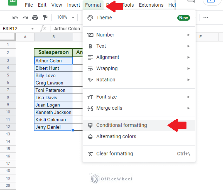
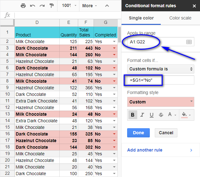
Web to format an entire row based on the value of one of the cells in that row: Click on format in the navigation bar, then select conditional formatting.. Select the range you want to format, for example, columns a:e. On your computer, open a spreadsheet in google sheets. You can use the custom formula function in google sheets to apply conditional formatting based on a cell value from another sheet. Select the cell you want to format. Conditional formatting from another sheet. Web below are the steps to do this: This functionality is called conditional formatting. Select the cells that you want to highlight (student’s names in this example) step 2:
Web conditional formatting based on another cell range 1. Click the format option step 3: On your computer, open a spreadsheet in google sheets. Select the cells that you want to highlight (student’s names in this example) step 2: This functionality is called conditional formatting. Click on format in the navigation bar, then select conditional formatting.. Select the range you want to format, for example, columns a:e. You can use the custom formula function in google sheets to apply conditional formatting based on a cell value from another sheet. This can be done based on the. Select the cell you want to format.
Conditional Formatting Based on Another Cell in Google Sheets OfficeWheel
Web conditional formatting based on another cell range 1. Web to format an entire row based on the value of one of the cells in that row: This can be done based on the. Conditional formatting from another sheet. On your computer, open a spreadsheet in google sheets.
How to Use Google Spreadsheet Conditional Formatting to Highlight
On your computer, open a spreadsheet in google sheets. Click the format option step 3: Web fortunately, with google sheets you can use conditional formatting to change the color of the cells you’re looking for based on the cell value. Click on format in the navigation bar, then select conditional formatting.. Select the range you want to format, for example,.
Conditional Formatting Based on Another Cell in Google Sheets OfficeWheel
This functionality is called conditional formatting. Select the cell you want to format. Select the cells that you want to highlight (student’s names in this example) step 2: Click the format option step 3: This can be done based on the.
Conditional Formatting Based on Another Cell in Google Sheets OfficeWheel
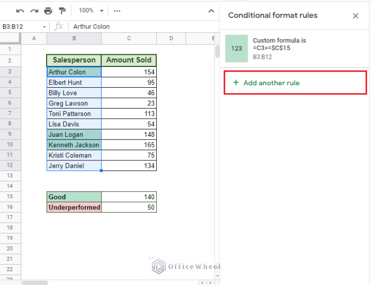
Select the cells that you want to highlight (student’s names in this example) step 2: Click on format in the navigation bar, then select conditional formatting.. Click the format option step 3: Web below are the steps to do this: On your computer, open a spreadsheet in google sheets.

Google sheets conditional formatting to colour cell if the same cell in
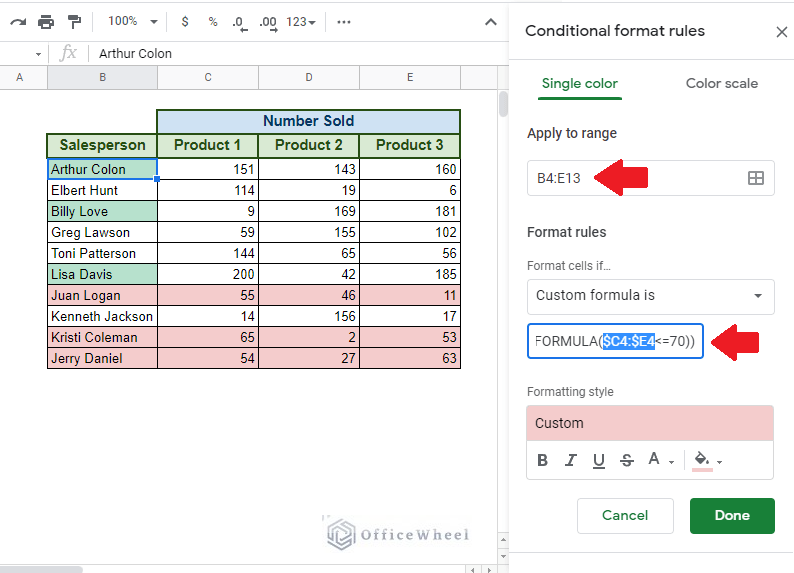
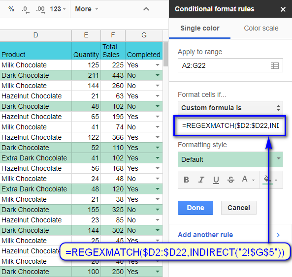
On your computer, open a spreadsheet in google sheets. You can use the custom formula function in google sheets to apply conditional formatting based on a cell value from another sheet. This can be done based on the. Web fortunately, with google sheets you can use conditional formatting to change the color of the cells you’re looking for based on.
Conditional Formatting Based on Another Cell in Google Sheets OfficeWheel
This can be done based on the. Web fortunately, with google sheets you can use conditional formatting to change the color of the cells you’re looking for based on the cell value. Click on format in the navigation bar, then select conditional formatting.. Select the range you want to format, for example, columns a:e. Click the format option step 3:
1 Cell Format All Rows Conditional Formatting
On your computer, open a spreadsheet in google sheets. Select the range you want to format, for example, columns a:e. Select the cells that you want to highlight (student’s names in this example) step 2: Web fortunately, with google sheets you can use conditional formatting to change the color of the cells you’re looking for based on the cell value..

Conditional Formatting in Google Sheets Guide 2023 Coupler.io Blog
Select the cell you want to format. You can use the custom formula function in google sheets to apply conditional formatting based on a cell value from another sheet. Click on format in the navigation bar, then select conditional formatting.. Web conditional formatting based on another cell range 1. Web below are the steps to do this:

Google Sheets Indirect Conditional Formatting Sablyan
Click the format option step 3: Select the cell you want to format. This can be done based on the. Web to format an entire row based on the value of one of the cells in that row: Conditional formatting from another sheet.

Conditional Formatting Based on Another Cell in Google Sheets OfficeWheel
Web fortunately, with google sheets you can use conditional formatting to change the color of the cells you’re looking for based on the cell value. Web to format an entire row based on the value of one of the cells in that row: On your computer, open a spreadsheet in google sheets. Conditional formatting from another sheet. Web below are.
Click The Format Option Step 3:
Web conditional formatting based on another cell range 1. This can be done based on the. Select the cell you want to format. Web fortunately, with google sheets you can use conditional formatting to change the color of the cells you’re looking for based on the cell value.
This Functionality Is Called Conditional Formatting.
Web below are the steps to do this: Select the cells that you want to highlight (student’s names in this example) step 2: You can use the custom formula function in google sheets to apply conditional formatting based on a cell value from another sheet. Web to format an entire row based on the value of one of the cells in that row:
On Your Computer, Open A Spreadsheet In Google Sheets.
Conditional formatting from another sheet. Click on format in the navigation bar, then select conditional formatting.. Select the range you want to format, for example, columns a:e.